Lecture 3 - Neural Networks & Deep Learning Foundations
Welcome back!
Last time: AI-assisted development + classical NLP (bag-of-words, n-grams)
Today: The machinery that makes it all work - neural networks and deep learning
Logistics:
- Today may be review (or not) - mixing it up
- Week numbering for assignments
- Last day for add/drop
Ice breaker
If you could go back in time, at what age would you have given yourself access to ChatGPT?
https://answergarden.ch/5123533
Agenda for today
- Neural networks review - the building blocks
- How learning works - backpropagation
- Training in practice + hands-on exploration
- Looking ahead: sequences and scale
The landscape of neural networks
| Architecture | Key idea | Used for |
|---|---|---|
| Feed-forward (MLP) | Data flows one direction | Classification, regression |
| CNN | Sliding filters | Images, spatial patterns |
| RNN | Memory through loops | Sequences (we'll see next week) |
| Transformer | Attention mechanism | LLMs (our goal!) |
Today: Feed-forward networks. The foundation for everything else.
Part 1: Neural Networks - The Building Blocks
The biological inspiration
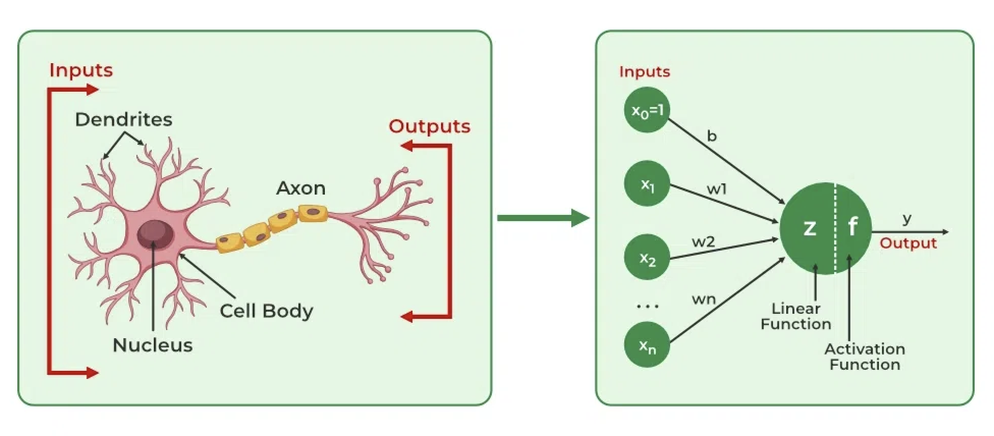
| Biological | Artificial |
|---|---|
| Dendrites receive signals | Inputs (numbers) |
| Cell body processes | Weighted sum + bias |
| Fires if threshold reached | Activation function |
| Axon outputs | Output value |
The analogy breaks down quickly, but it remains an inspiration for network design
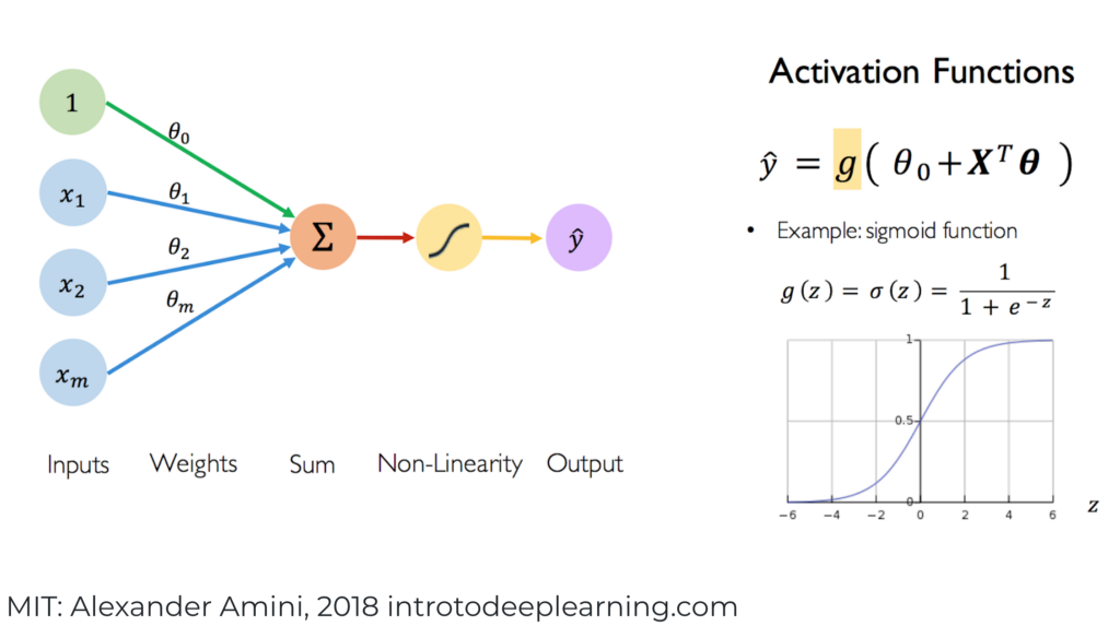
A single artificial neuron
| Component | Role |
|---|---|
| Inputs | Data coming in |
| Weights | Learned importance of each input |
| Bias b | Learned offset |
| Activation f | Introduces non-linearity |
Activation functions - why we need them
Without activation (just linear combinations):
Multiple layers = still just one linear transformation!
With activation (non-linearity):
We can approximate any function!
This is the key to deep learning's power
Quick thought experiment
What would happen if we removed ALL activation functions from a 10-layer network?
Answer: It collapses to a single linear transformation. Ten layers of matrix multiplication = one matrix multiplication. All that depth buys you nothing without non-linearity!
Common activation functions
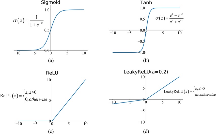
| Function | Formula | Range | Notes |
|---|---|---|---|
| Sigmoid | Probabilities; vanishing gradients | ||
| Tanh | Zero-centered; used in RNNs | ||
| ReLU | Modern default; fast & simple | ||
| Leaky ReLU | Fixes "dying ReLU" problem |
Multi-layer networks
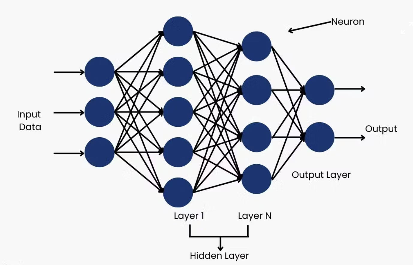
- Input layer: Your features (e.g., word embeddings)
- Hidden layers: Where the magic happens
- Output layer: Your prediction
Each layer transforms the representation
It's just an equation
A neural network is just a big equation with many parameters
Single neuron:
One hidden layer (vector form):
Two hidden layers:
GPT-5 (~10T parameters): Same pattern, just... more.
Familiar friends in disguise
Linear regression is a neural network:
- 0 hidden layers
- No activation function
- y = Wx + b
Logistic regression is a neural network:
- 0 hidden layers
- Sigmoid activation
- y = σ(Wx + b)
Large networks generalize from here
Using NNs: Forward propagation
- Start with inputs
- Multiply by weights, add bias
- Apply activation function
- Repeat for each layer
- Get prediction at output
This is just matrix multiplication + activation!
Think-pair-share: Why go deep?
Question: Why use multiple hidden layers instead of one giant layer?
Why depth matters
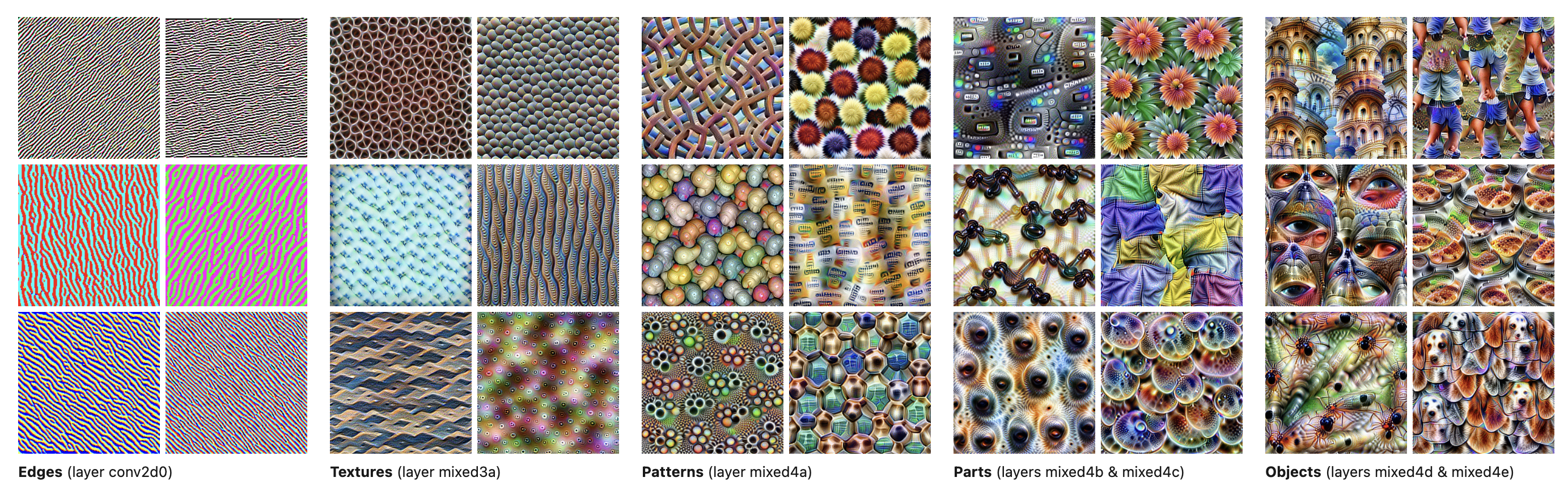
Deep networks learn hierarchical representations
Why depth matters
Example: Learning word embeddings
Layer 1: Character patterns (prefixes, suffixes, common letter combinations)
Layer 2: Syntactic roles (noun vs verb, singular vs plural)
Layer 3: Semantic clusters (animals, emotions, actions)
This is how neural networks learn rich representations: each layer builds on the previous.
Part 2: How Learning Works - Backpropagation
The learning problem
We have:
- Network with random initial weights
- Training data (input, correct output)
We want:
- Adjust weights so predictions match correct outputs
But how do we know what "match" means?
Learning as optimization
Key insight: Frame learning as minimization
We need two things:
| Component | Question it answers |
|---|---|
| Loss function | How wrong are we? (a single number) |
| Optimization method | How do we find better weights? |
The recipe:
- Make a prediction
- Measure how wrong we are (loss)
- Adjust weights to reduce loss
- Repeat
Quick chat: What's "wrong"?
Turn to a neighbor: How would you measure "wrongness" for each task?
| Task | What number captures how wrong we are? |
|---|---|
| Predicting house prices | ? |
| Detecting cancer in scans | ? |
| Predicting star ratings (1-5) | ? |
| Recommending chess moves | ? |
| Generating images from a prompt | ? |
Gradient descent intuition
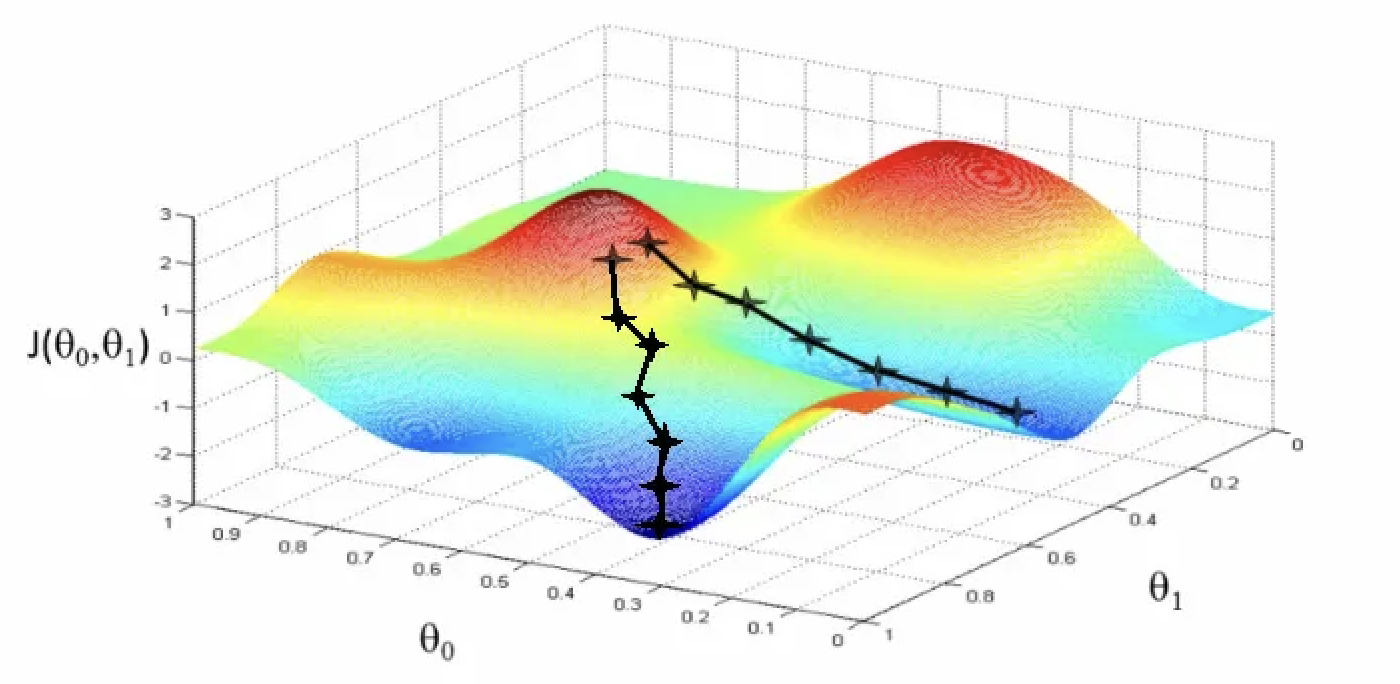
Imagine: Lost in foggy mountains, trying to reach the valley
Strategy: Feel the slope under your feet, step downhill
Repeat: Until you can't go lower
The reality:
Gradient descent: the math
Gradient: Vector pointing in direction of steepest increase
We want to go downhill, so we go the opposite direction:
Where (eta) is the learning rate
Learning rate matters
Draw on the board:
Too small: Takes forever, might get stuck
Too large: Overshoot the minimum, bounce around or diverge
Just right: Converge efficiently to minimum
In practice: Start with 0.001, adjust based on training curves
Stochastic Gradient Descent (SGD)
Full gradient descent: Compute gradient using ALL training examples
Problem: N might be millions. One step = one pass through entire dataset!
Stochastic GD: Use a random mini-batch of examples instead
Typical batch sizes: 32, 64, 128, 256
The answer is counterintuitive:
- Speed tradeoff: Each step is noisier, but we can take many more steps
- Noise is a feature: Random kicks help escape local minima and saddle points
- Regularization effect: The noise actually improves generalization
- Practical necessity: GPU memory can only fit a batch, not millions of examples
This is what everyone actually uses (usually with Adam optimizer on top)
But how do we compute gradients?
Problem: Our network has thousands/millions of parameters
Question: How does changing one weight affect the final loss?
Answer: The chain rule from calculus!
This is backpropagation
Backpropagation - the key insight
Forward pass: Input -> Layer 1 -> Layer 2 -> Output -> Loss
Backward pass: Propagate error information backward through the network
The manager metaphor
Chain rule: If A affects B, and B affects C, then:
Backprop is just an efficient way to apply the chain rule
Loss functions - measuring wrongness
Loss function: A single number telling us how wrong we are
Higher loss = worse predictions
Goal: Find parameters that minimize loss
Mean Squared Error (MSE)
For regression (predicting continuous values):
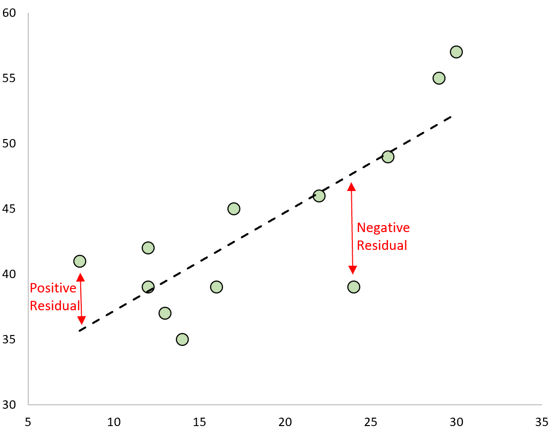
Intuition: Penalize distance from correct answer, squared
Why squared?
- Differentiable everywhere (no absolute value kink)
- Bigger errors hurt more than small errors
Example: Predicting house prices, temperature, stock prices
Cross-Entropy Loss
For classification (predicting categories):
Where y is true label (one-hot), ŷ is predicted probabilities
Binary case: L = -[y log(ŷ) + (1-y) log(1-ŷ)]
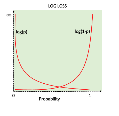
Intuition: Punish confident wrong predictions severely
Softmax: from scores to probabilities
Before cross-entropy, we need probabilities. Softmax converts raw scores to probabilities:
Properties:
- All outputs between 0 and 1
- All outputs sum to 1
- Preserves ordering (highest score -> highest probability)
- Differentiable!
Example: Scores [2.0, 1.0, 0.1] -> Probabilities [0.66, 0.24, 0.10]
KL Divergence (preview)
Kullback-Leibler divergence: How different are two probability distributions?
Not symmetric:
Cross-entropy = KL divergence + constant (when P is fixed)
Where you'll see it:
- Training LLMs (comparing predicted vs actual next-word distributions)
- Variational autoencoders
- Knowledge distillation (making smaller models mimic bigger ones)
Loss functions must be differentiable
Why? We need to compute gradients!
tells us how to adjust weights
If loss has "kinks" or discontinuities:
- Can't compute gradient at those points
- Optimization gets stuck or behaves badly
This is why we use:
- Squared error (not absolute error)
- Cross-entropy (not 0/1 accuracy)
- Smooth activation functions (or ReLU, which is "almost" smooth)
Backprop example: setup
Tiny network: 1 input, 1 hidden, 1 output
| Value | |
|---|---|
| Input x | 2 |
| Weight | 0.5 |
| Weight | 1.0 |
| Target y | 3 |
| Activation | ReLU |
| Loss | MSE |
Backprop example: forward pass
Step through the computation:
1
1
4
We predicted 1, target was 3. Loss = 4.
Now: how should we adjust and to reduce loss?
Backprop example: backward pass
Apply chain rule, working backward:
Gradient is -4: Increasing would decrease loss (good!)
Backprop example: the update
Update rule:
With learning rate :
Sanity check: New prediction would be
Closer to target of 3! Loss would drop from 4 to 2.56.
Repeat thousands of times -> weights converge to good values
PyTorch does the math for you
You never write gradient code. Frameworks handle backprop automatically.
import torch

# Define network
model = torch.nn.Sequential(
    torch.nn.Linear(10, 5),
    torch.nn.ReLU(),
    torch.nn.Linear(5, 1)
)

# Forward pass - you write this
prediction = model(x)
loss = (prediction - target) ** 2

# Backward pass - PyTorch does this automatically!
loss.backward()

# Update weights
optimizer.step()
The magic: .backward() applies the chain rule through your entire network
This is why we can train models with billions of parameters
Training loop - putting it together
Repeat many times:
- Forward pass - compute predictions
- Compute loss
- Backward pass - compute gradients
- Update weights
Over many iterations: Loss goes down, predictions improve!
Explain it to a friend
Pair up: Pretend your partner knows nothing about deep learning.
Explain how a neural network learns in plain language. What's actually happening?
Part 3: Training in Practice
Hyperparameters matter
Learning rate: How big are the steps?
- Too large: overshoot the minimum, diverge
- Too small: takes forever, gets stuck
Batch size: How many examples before updating?
- Larger: more stable, slower
- Smaller: noisier, faster, better generalization
Network architecture: How many layers? How many nodes?
Activation functions, initialization, optimization algorithm...
It's an art and a science
Beyond vanilla gradient descent
Vanilla gradient descent: w_new = w_old - learning_rate × gradient
Problem: Uses fixed learning rate, treats all parameters the same
Adam optimizer (Adaptive Moment Estimation):
- Keeps moving averages of gradients and squared gradients
- Adjusts learning rate for each parameter individually
- Fast convergence, works well in practice
Why it matters: Adam is the default optimizer for most modern deep learning (including training LLMs!)
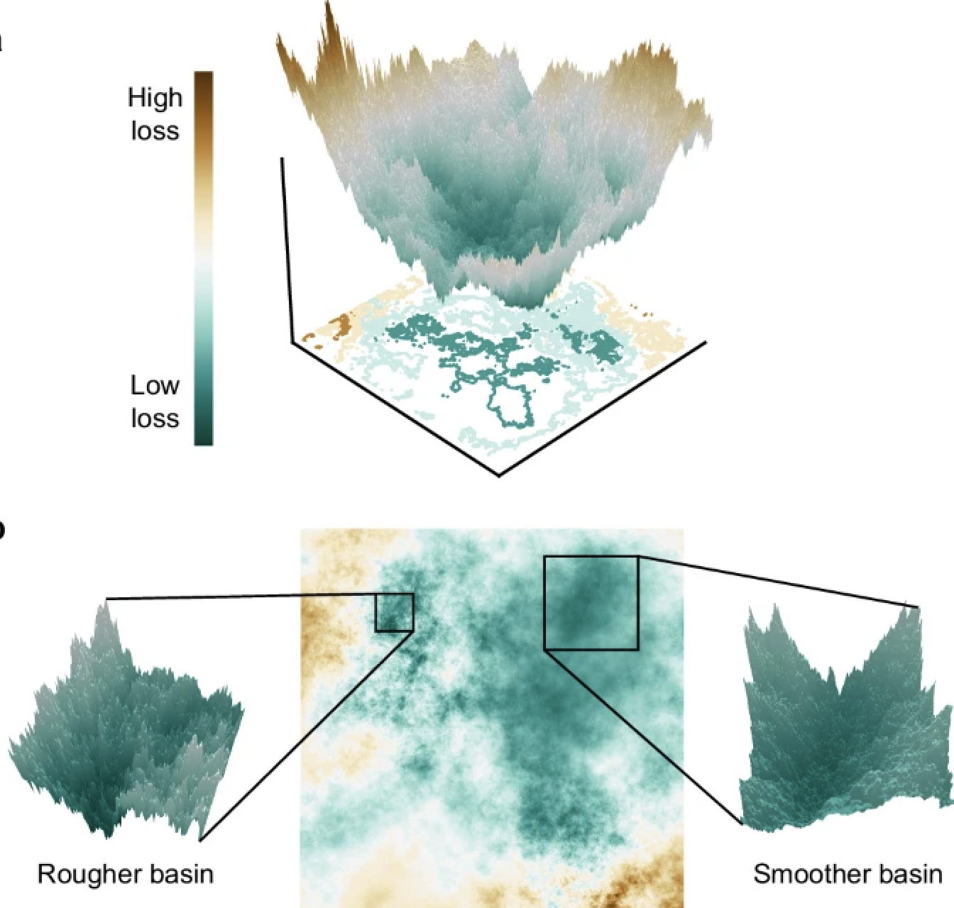
Common challenges
Vanishing gradients: Gradients get tiny in deep networks
Exploding gradients: Gradients get huge, weights blow up
Overfitting: Memorizes training data, fails on new data
Local minima: Gets stuck in suboptimal solutions
Solutions: Better architectures (ReLU, skip connections), regularization, careful initialization
Topics to explore on your own
These are important but we won't cover in depth:
| Topic | One-liner |
|---|---|
| Regularization (L1, L2) | Penalize large weights to prevent overfitting |
| Dropout | Randomly "turn off" neurons during training |
| Batch normalization | Normalize layer inputs for stable training |
| Early stopping | Stop training when validation loss stops improving |
| Learning rate schedules | Decrease learning rate over time |
| Weight initialization | How you start matters (Xavier, He init) |
| Gradient clipping | Cap gradients to prevent explosion |
Activity: TensorFlow Playground
Open: playground.tensorflow.org
Try to classify the spiral dataset with:
- Just 1 hidden layer. Can you do it?
- Using linear activation instead of ReLU - what changes?
- What happens if you sent a very large or very small learning rate?
Let's add some competition: Find the SMALLEST network (fewest total neurons) that achieves loss < 0.1 on spiral.
Part 4: Looking Ahead - Sequences and Scale
What we've covered so far
Week 2: Classical NLP (bag-of-words, n-grams) and AI-assisted development
Today: How neural networks learn (backprop, gradient descent)
Wednesday: Tokenization - how text becomes input for these networks
Next challenge: How do we apply neural networks to sequences?
The problem with feed-forward networks
Feed-forward networks expect:
- Fixed-size input
- Fixed-size output
- No memory of previous inputs
But text is:
- Variable length
- Sequential (order matters!)
- Context-dependent
Examples of sequence tasks
Machine translation: Variable length in, variable length out
"Hello" -> "Bonjour"
"How are you?" -> "Comment allez-vous?"
Sentiment analysis: Variable length in, single output
"This movie was amazing!" -> Positive
Text generation: Sequence in, next word out
"The cat sat on the" -> "mat"
Feed-forward networks can't handle these naturally
Why variable length is hard
Traditional approach:
- Pad all sequences to max length (wasteful)
- Or truncate long sequences (lose information)
Either way, we lose the "sequential" aspect
We need architectures designed for sequences
Long-range dependencies
Remember this? "The trophy would not fit in the suitcase because it was too large"
What is "it"? The trophy or the suitcase?
Answer: The trophy (because it was too large)
Challenge: "it" is far from "trophy" in the sequence
Feed-forward networks treat each position independently
What we need for sequences
Memory: Remember what came before
Flexible length: Handle any input/output size
Order awareness: Position matters!
Context: Use earlier words to understand later ones
The evolution of solutions
1990s-2000s: Statistical machine translation (word alignment tables, phrase tables)
2014-2017: RNNs and LSTMs (memory in hidden states) - Monday
2017-present: Transformers with attention - Wednesday
Each approach solved some problems but had new limitations
The scale of modern deep learning
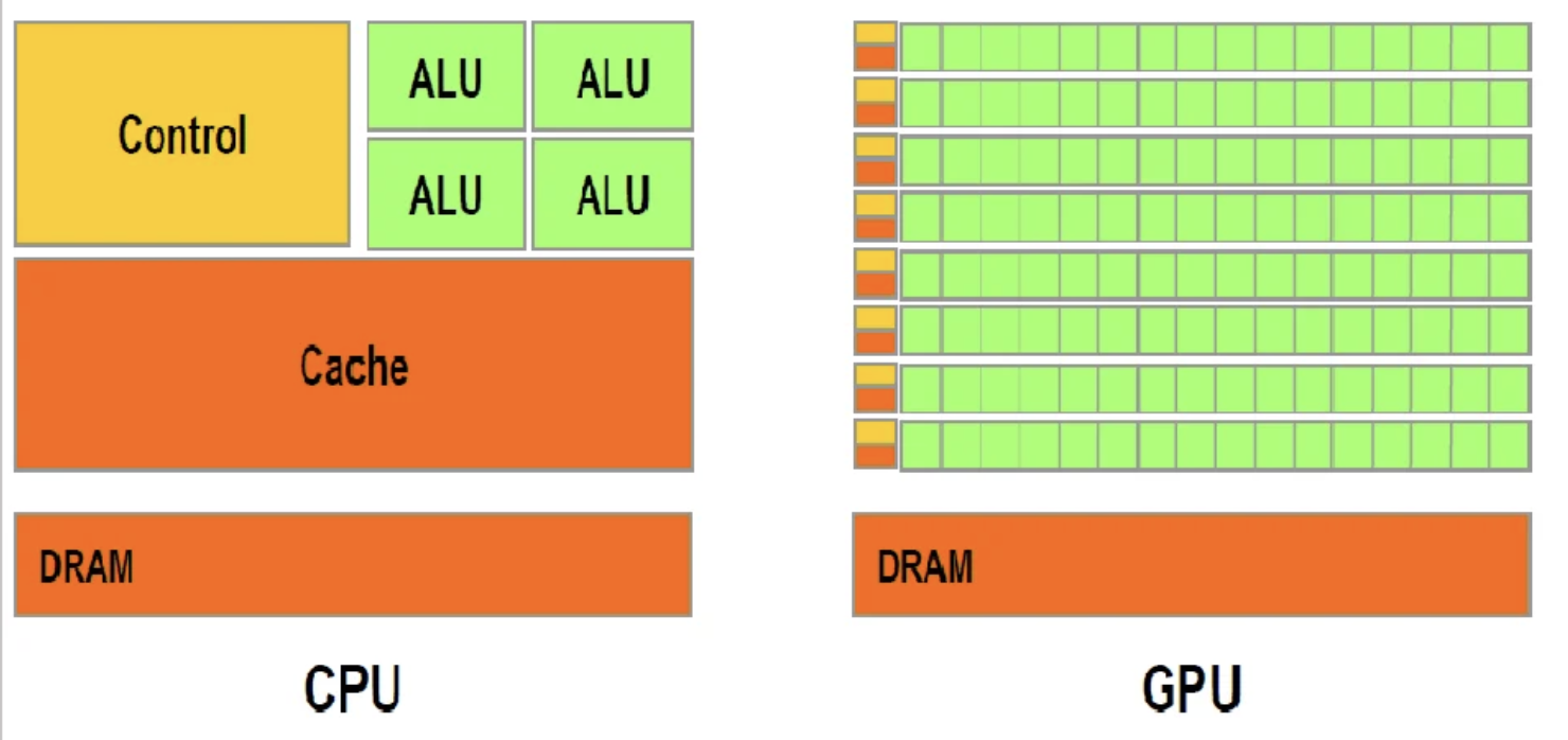
Training neural networks is mostly matrix multiplication
| CPU | GPU |
|---|---|
| 4-16 powerful cores | Thousands of simple cores |
| Great at complex sequential tasks | Great at simple parallel tasks |
Why GPUs? Matrix multiplication is perfectly parallelizable
The result: Training that would take months on CPUs takes days on GPUs
The cost of scale
| Model | Parameters | Est. Training Cost | Est. CO2 (tons) |
|---|---|---|---|
| GPT-3 (2020) | 175B | ~$4.6M | ~552 |
| GPT-4 (2023) | ~1.8T | ~$78-100M | ~12,500-15,000 |
| Claude 3.5 Sonnet | undisclosed | "tens of millions" | undisclosed |
| Gemini Ultra | undisclosed | ~$191M | undisclosed |
| Llama 3.1 405B | 405B | ~$640M | undisclosed |
| DeepSeek V3 | 671B (37B active) | ~$5.6M* | undisclosed |
| Grok 3 | undisclosed | ~$2-3B | undisclosed |
*Caution: These figures aren't directly comparable. Eg. DeepSeek's $5.6M is compute-only; Grok's $2-3B includes buying 100K GPUs.
Putting it in context:
| Activity | CO2 (tons/year) | Equivalent to... |
|---|---|---|
| Training GPT-4 (once) | ~12,500-15,000 | ~3,000 cars for a year |
| Bitcoin mining | ~40-98 million | 10-25% of all US cars |
| All US passenger cars | ~370 million | - |
Training is just the beginning. Using the model (inference) now accounts for more than half of total lifecycle emissions.
Discussion: Who bears the cost?
Turn to your neighbor:
-
Training large models requires massive compute resources. Who has access to this? Who doesn't?
-
The environmental cost is real. Should there be regulations on AI training? Who should decide?
-
Is it ethical to train ever-larger models? What are the trade-offs?
What we've learned today
Neural networks: Layers of weighted sums + activation functions
Learning: Gradient descent to minimize loss, backprop to compute gradients
Training: Hyperparameters matter, GPUs enable scale
Looking ahead: Sequences are hard (variable length, memory, context)
The bigger picture: Scale has costs - computational, financial, environmental
Reminders
Lab/Reflection due Friday (Feb 6): Tokenization and Neural Network Basics
You'll get to explore tokenization and building simple neural networks. Today's lecture gives you the foundation for the neural network part.
See the Week 3 guide for suggested explorations and resources
Wednesday (Feb 4): Tokenization - how text becomes numbers for neural networks