Lecture 15 - Retrieval-Augmented Generation (Part 1)
Ice breaker
Do you ever ask LLMs about current/recent events? How does it go?
Today's plan
- The context problem: why LLMs need help
- RAG architecture: retrieve, augment, generate
- Chunking strategies
- Vector databases and semantic search
- Re-ranking and hybrid search
Part 1: The Context Problem
LLMs have a knowledge problem
1. Knowledge cutoff
- Models trained on data up to certain date, don't know recent events
2. Hallucination on specifics
- Make up facts confidently, especially on niche topics, specific details (dates, names, links)
3. No access to private data
- Can't see external documents and data, only know public training data
4. Context window limits
- Even high context limits are finite, and suffer from decay
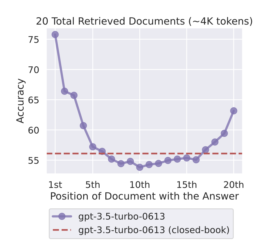
Context window: the "lost in the middle" problem
More context doesn't always mean better answers.
Liu et al. (2023): performance drops significantly for information buried in the middle of a long context. Models attend far more to the start and end.
Rule of thumb: Put your most important content first or last. (We saw this in Week 7 - and it's one reason RAG outperforms "just stuff everything in context.")
Traditional solutions and their trade-offs
What's the problem with each of these?
Option 1: Put everything in the prompt
- Problems: token limits, cost, missing middle, lack of structure
Option 2: Fine-tune the model on your data
- Problems: expensive, slow, doesn't fix hallucinations
Option 3: Use filtering and human review to validate
- Problems: not scalable, slow, expensive
We need a better solution!
Introducing RAG: Retrieval-Augmented Generation
RAG = Retrieve + Augment + Generate
Don't put everything in the prompt. Just put the relevant parts.
Step 1: Retrieval Find relevant documents for the query
Step 2: Augmentation Add retrieved docs to prompt as context
Step 3: Generation LLM generates answer grounded in retrieved context
RAG Example and Why it Works
Example:
User question: "What is our company's vacation policy?"

1. RETRIEVE: Search company handbook, find section on vacation policy
2. AUGMENT: Create prompt: "Based on these documents: [vacation policy text],
            answer: What is the vacation policy?"
3. GENERATE: LLM reads context and answers accurately
Why this works:
- Only relevant context in prompt (efficient, fits in context)
- LLM answers from documents, not from weights (reduces hallucination)
- Can cite sources (show which document answer came from)
- Easily updatable (don't have to retrain the model)
- Works with sensitive data (data kept strictly separate from the model)
- Much cheaper than fine-tuning (just pay for retrieval and LLM compute/API calls)
For a deeper dive: The original RAG paper (Lewis et al., 2020)
Part 2: RAG Architecture
RAG architecture diagram
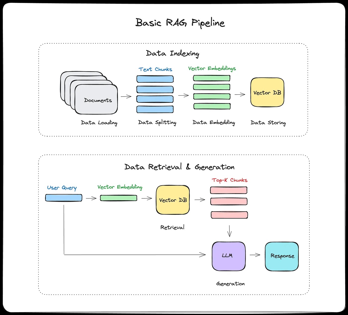
The RAG pipeline steps
Offline (indexing, done once):
- Split documents into chunks
- Generate embeddings for each chunk
- Store in vector database
Online (for every query):
- User asks question
- Generate embedding for question
- Search vector DB for similar chunks
- Add top chunks to LLM prompt
- LLM generates answer
- Return answer + sources
When does RAG help?
RAG excels at:
- Q&A over documents
- Chatbots with knowledge base
- Research assistants
- Customer support (search FAQs + docs)
Especially for:
- Factual questions
- Large knowledge bases (won't fit in context)
- Frequently updated information
- Private/proprietary data
Fine-tuning vs RAG
RAG won't help you with:
- Creative tasks (writing, brainstorming)
- Reasoning without facts
- Consistent style/voice
Consider fine-tuning instead if:
- Need consistent behavior/style
- Small, stable knowledge domain
- Want model to "internalize" knowledge
RAG + Fine-tuning:
- Fine-tune for style/behavior
- RAG for factual knowledge
- Best of both worlds (but more complex)
Example: Customer support bot
- Fine-tune: Learn company's friendly, helpful tone
- RAG: Look up specific product info, policy details
What can go wrong at each step?
Part 3: Chunking Strategies
Chunking: The most important decision in RAG
Your chunks are what the retriever can find.
- If a chunk is too big, it's full of irrelevant text.
- Too small, it's missing context.
Everything downstream depends on this.
What bad chunking looks like
Original document:
...The standard dosage is 500mg twice daily. Patients with
renal impairment should reduce to 250mg once daily.

CONTRAINDICATIONS: Do not prescribe to patients with a
history of liver disease or those currently taking warfarin...
Naive split (no overlap, fixed at 30 tokens):
Chunk 1: "...standard dosage for xyz is 500mg twice daily.
          Patients with renal impairment should reduce to"

Chunk 2: "250mg once daily. CONTRAINDICATIONS: Do not
          prescribe to patients with a history of"

Chunk 3: "liver disease or those currently taking warfarin..."
Query: "Can I prescribe xyz to a patient on warfarin?"
What are some issues here?
Chunking Strategies
Fixed-size chunking:
- 200-500 tokens per chunk
- 10-20% overlap between chunks
- Simple, predictable, works well as a default
Sentence-based:
- Split at sentence boundaries
- Group 3-5 sentences per chunk
- Preserves semantic units
Document-structure-aware:
- PDFs: chunk by page or section
- Code: chunk by function or class
- HTML: chunk by heading hierarchy
- Best when your documents have clear structure
Semantic chunking:
- Detect topic changes with embeddings and split there
- Higher quality results, but computationally expensive
Recommendation: Start with fixed-size (400-600 tokens, 20% overlap). Adjust based on your documents and retrieval quality.
Think about the medical document example from earlier. Which strategy would you pick for that, and why?
What good overlaps look like
Chunk 1: "The company was founded in 2015. Our mission is to
          make AI accessible. We started with three employees."

Chunk 2: "We started with three employees. By 2020, we had
          grown to 500 people across four offices."

Chunk 3: "...grown to 500 people across four offices. Our
          engineering team is based in Boston."
Overlap means a sentence at the boundary appears in both chunks, so the retriever can find it no matter which chunk it lands in.
Part 4: Vector Databases and Semantic Search
Why vectors? The problem with keyword search
Traditional keyword search:
- "dog" matches documents with word "dog"
- Doesn't match "puppy," "canine," "golden retriever"
- "Bag of words" approach limits meaningfulness
Semantic search:
- Understands meaning, not just words
- "dog" matches "puppy," "pet," related concepts
Semantic search with vectors:
Query: "dog training"
Embedding: [0.2, 0.8, -0.3, ..., 0.5]  (dense vector)

Similar documents:
- "puppy obedience classes" (high similarity)
- "teaching your canine commands" (high similarity)
- "pet behavior modification" (medium similarity)
This should seem pretty familiar by now...
- We created word and sentence vectors in Word2Vec
- And this is how we match queries and keys in attention
Vector databases: Making search fast
Why not just store embeddings in NumPy arrays?
- Millions of documents means billions of vector comparisons
- Brute force is too slow
Solution: Approximate Nearest Neighbor (ANN) search
- Don't compare against every vector, use smart data structures to narrow the search
- Trade a small amount of accuracy for a huge speedup
- Common algorithms: HNSW (graph-based, most popular), IVF (cluster-based), Product Quantization (compression)
- We'll look at how HNSW works on Wednesday
Popular tools:
- ChromaDB (local, easy)
- Pinecone (managed cloud)
- Weaviate (open source, scalable)
- FAISS (Facebook AI similarity search, library not DB)
- Others: Qdrant, Milvus, pgvector (Postgres extension)
ChromaDB in practice
import chromadb

# Create client and collection
client = chromadb.Client()
collection = client.create_collection("my_docs")

# Add documents
collection.add(
    documents=["This is doc 1", "This is doc 2"],
    ids=["doc1", "doc2"]
)

# Query
results = collection.query(
    query_texts=["document about X"],
    n_results=2
)
print(results)
Why does this look so easy?
There are powerful defaults
collection.addis running tokenization and a default embedding model,all-MiniLM-L6-v2, a Sentence Transformers modelcollection.queryuses a similarity metric (L2 by default, but you can change) it and uses HNSW for search
Demo: Querying a handbook
Let's load 10 chunks from a coffee shop employee handbook into ChromaDB and search them.
As we go, think about:
- Does the ranking match your intuition?
- Can you write a query that matches semantically but shares no keywords with the target?
- Can you write one that needs info from two chunks?
We'll come back to the challenge questions at the end if we have time.
Similarity metrics: How to compare vectors
Cosine similarity:
- Measures angle between vectors
- Range: -1 (opposite) to 1 (identical)
- Most common for text
Dot product:
- Sum of element-wise multiplication
- Faster than cosine (un-normalized cosine)
Euclidean distance (L2):
- Geometric distance between points
- Less common for text (more common for images)
- Can be affected by vector magnitude
Part 5: Semantic Search Deep Dive
The retrieval process step-by-step
Step 1: Embed the query
query = "What's the refund policy?"
query_embedding = embedding_model.encode(query)
# Returns: array of shape (384,) or (1536,) depending on model
Step 2: Similarity search in vector database
results = vector_db.search(
    query_vector=query_embedding,
    top_k=10,  # retrieve top 10 most similar chunks
    min_similarity=0.7  # optional: filter by similarity threshold
)
# Returns: [(chunk_id, similarity_score, metadata), ...]
Step 3: (Optional) Re-ranking
- First-pass retrieval: fast but approximate (top 10-20)
- Second-pass re-ranking: more expensive but accurate
- Use cross-encoder model to re-score retrieved chunks
- Reorder by new scores, keep top k (typically 3-5)
Step 4: Return top chunks with metadata
top_chunks = [
    {
        "text": "Our refund policy allows returns within 30 days...",
        "source": "refund_policy.pdf",
        "page": 3,
        "similarity": 0.89
    },
    # ... more chunks
]
Step 5: Format for LLM prompt (more next lecture)
context = "\n\n".join([chunk["text"] for chunk in top_chunks])
prompt = f"""Based on the following documents:

{context}

Answer this question: {query}"""
Re-ranking: Improving retrieval quality
Problem: First-pass retrieval is approximate
- Might retrieve some irrelevant chunks
- Might rank less-relevant chunks higher
Solution: Two-stage retrieval
- Fast retrieval (bi-encoder): Get top 10-20
- Accurate re-ranking (cross-encoder): Reorder, keep top 3-5
Bi-encoder (initial retrieval):
- General-purpose embedding model (e.g. MiniLM)
- Encodes query and doc separately, compares vectors
- Fast: pre-compute doc embeddings, just do cosine similarity at query time
Cross-encoder (re-ranking):
- Specially trained on relevance datasets (e.g. MS MARCO, millions of query-passage pairs labeled relevant/not)
- Concatenates input as
[CLS] query [SEP] doc [SEP]and feeds through transformer - Cross-attention between query and doc tokens at every layer, so it sees word-level interactions
- Outputs a single relevance score, not an embedding
- More accurate, but must run once per document, so only practical on small sets (10-20 docs)
When to use re-ranking:
- High-stakes applications (legal, medical)
- When retrieval quality is critical
- Acceptable to add ~100ms latency
- Production systems often use this
What's the trade-off you're making by adding a re-ranking step? When would it not be worth it?
Re-ranking in practice
Stage 1: Fast retrieval (bi-encoder)
query_emb = embed(query)
doc_embs = [embed(doc) for doc in corpus]
top_10 = find_most_similar(query_emb, doc_embs, k=10)
- Fast: pre-compute doc embeddings once, just compare vectors
- Gets good candidates but not perfect ranking
Stage 2: Re-ranking (cross-encoder)
scores = []
for doc in top_10:
    # Cross-encoder sees query + doc together
    score = cross_encoder.predict([query, doc])
    scores.append(score)

# Re-sort by cross-encoder scores
top_3 = sort_by_score(top_10, scores)[:3]
Semantic search + Keyword search = Hybrid search
- Semantic search is great for concepts, paraphrasing, understanding meaning
- Keyword search (BM25) is great for exact terms, proper names, IDs
- Each has strengths and weaknesses, so combine them
Example query: "GPT-4 performance on math benchmarks"
Semantic search retrieves:
- Documents about LLM mathematical reasoning capabilities
- Papers on model evaluation and testing
Keyword search retrieves:
- Documents that specifically mention "GPT-4" (exact match)
- Papers with "benchmark" in the title
Hybrid search retrieves:
- Best of both: documents that are semantically relevant AND contain key terms
When to use hybrid:
- Queries with specific terms, names, IDs
- Domain where exact matches matter (legal, medical, technical)
- Want robust retrieval across query types
If you were building a RAG system for BU's course catalog, would you use semantic search, keyword search, or hybrid? Think about the kinds of queries students would ask.
Reciprocal Rank Fusion (RRF)
Problem with combining scores directly:
- Semantic search returns distances (lower = better, unbounded)
- BM25 returns relevance scores (higher = better, 0 to ~25+)
- Different scales, different directions, can't just average them
RRF sidesteps this by combining ranks, not scores:
- is a smoothing constant (typically 60)
- is where document appeared in retriever 's results
- A doc ranked #1 in both lists gets: 1/(60+1) + 1/(60+1) = 0.033
- A doc ranked #1 in one, #10 in the other: 1/(60+1) + 1/(60+10) = 0.031
Why ranks work better than scores:
- No normalization needed
- Robust to outlier scores
- Works even when retrievers return completely different score distributions
- Simple to implement, hard to beat in practice
Hybrid search in practice
Implementation with RRF:
import chromadb
from rank_bm25 import BM25Okapi
import numpy as np

docs = ["Our refund policy allows returns within 30 days",
        "Contact support at help@company.com",
        "Shipping takes 5-7 business days"]
ids = ["doc1", "doc2", "doc3"]

# Semantic search with ChromaDB
client = chromadb.Client()
collection = client.create_collection("my_docs")
collection.add(documents=docs, ids=ids)

query = "how do I get my money back?"
semantic_results = collection.query(query_texts=[query], n_results=3)
sem_ranking = semantic_results["ids"][0]  # ordered by distance

# Keyword search with BM25
tokenized_docs = [doc.lower().split() for doc in docs]
bm25 = BM25Okapi(tokenized_docs)
bm25_scores = bm25.get_scores(query.lower().split())
bm25_ranking = [ids[i] for i in np.argsort(-bm25_scores)]  # sort descending

# Reciprocal Rank Fusion
k = 60
rrf_scores = {}
for ranking in [sem_ranking, bm25_ranking]:
    for rank, doc_id in enumerate(ranking, start=1):
        rrf_scores[doc_id] = rrf_scores.get(doc_id, 0) + 1 / (k + rank)

final_ranking = sorted(rrf_scores, key=rrf_scores.get, reverse=True)
If time, we can return to the python notebook
Wrapping up
Key takeaways
1. RAG addresses key LLM limitations:
- Knowledge cutoff (add recent docs)
- Hallucination (ground in retrieved facts)
- Private data (search your own documents)
- Context limits (retrieve only relevant parts)
2. Three-stage pipeline:
- Retrieve: Find relevant chunks from vector database
- Augment: Add chunks to prompt as context
- Generate: LLM answers using context
3. Vector databases enable semantic search:
- Embeddings = dense numerical representations
- Similar meanings, similar vectors
- Fast approximate nearest neighbor search (HNSW, IVF)
- ChromaDB, Pinecone, Weaviate are popular options
4. Retrieval can be sophisticated:
- Re-ranking: bi-encoder for speed, cross-encoder for accuracy
- Hybrid search: combine semantic + keyword with RRF
- Tunable parameters: chunk size, overlap, top k, similarity threshold
5. Next lecture: Prompt engineering for RAG, how vector search works under the hood, security, and evaluation
Coming up
Wednesday (Apr 1):
- Prompt engineering for RAG
- Advanced techniques: contextual retrieval, HyDE, query routing
- How vector search actually works (HNSW)
- Security and failure modes
- Evaluating RAG systems
Lab due this week on RAG